


I used to work with BERT and its siblings but I never paid a lot of attention to “what it actually is”. I’ve decided to fill this shameful gap in my knowledge and build at least its minimal working version. Searching for the tutorial didn’t help me much, I had to gather the knowledge in little pieces to get a full picture of BERT.
This article is my attempt to create a thorough tutorial on how to build BERT architecture using PyTorch.
The full code to the tutorial is available at pytorch_bert.
Long Story Short about BERT
BERT stands for Bidirectional Encoder Representation from Transformers. The original BERT: Pre-training of Deep Bidirectional Transformers for Language Understanding, actually, explains everything you need to know about BERT.
Honestly saying, there are much better articles on the Internet explaining what BERT is, for example, BERT Explained: State of the art language model for NLP. After reading this article, you may have some questions about attention mechanisms; this article Illustrated: Self-Attention explains attentions.
In this paragraph I just want to run over the ideas of BERT and give more attention to the practical implementation.
BERT solves two tasks simultaneously:
- Next Sentence Prediction (NSP) ;
- Masked Language Model (MLM).
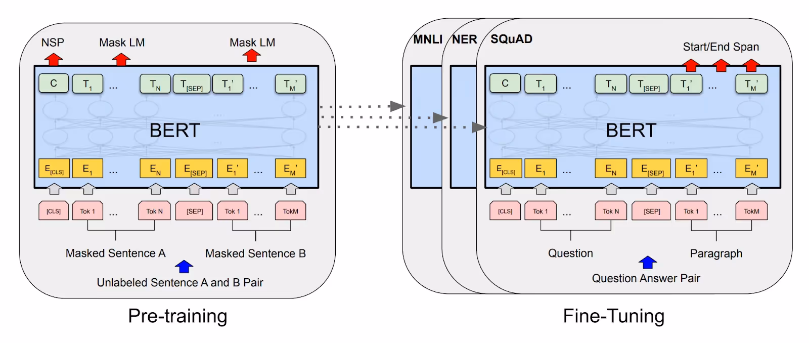
Next Sentence Prediction
NSP is a binary classification task. Having two sentences in input, our model should be able to predict if the second sentence is a true continuation of the first sentence.
For example, there is a paragraph
I have a cat named Tom. Tom likes to play with birds sitting on the window.
They like this game not. I also have a dog. We walk together everyday.
The potential dataset will look like
| Sentence | NSP class |
|---|---|
| I have a cat named Tom. Tom likes to play with birds sitting on the window | is next |
| I have a cat named Tom. We walk together everyday | is not next |
Masked Language Model
Masked Language Model is the task to predict the hidden words in the sentence.
For example, having a sentence
Tom likes to [MASK] with birds [MASK] on the window.
the model should predict that masked words are play and sitting.
Building BERT
To build BERT we need to work out three steps:
- Prepare Dataset;
- Build a model;
- Build a trainer.

Prepare Dataset
In the case of BERT, the dataset should be prepared in a certain way. I spent maybe 30% of the time and my brain power only to build the dataset for the BERT model. So, it’s worth a discussion in its own paragraph.
The original BERT uses BooksCorpus (800M words) and English Wikipedia (2,500M words) for pre-training. We use IMDB reviews data with ~72k words.
Download the dataset from Kaggle: IMDB Dataset of 50K Movie Reviews and put it under data/ directory in the root of your project.
Following, pytorch’s DATASETS & DATALOADERS we have to create Dataset that extends torch.utils.data.Dataset class.
class IMDBBertDataset(Dataset):
    # Define Special tokens as attributes of class
    CLS = '[CLS]'
    PAD = '[PAD]'
    SEP = '[SEP]'
    MASK = '[MASK]'
    UNK = '[UNK]'

    MASK_PERCENTAGE = 0.15  # How much words to mask

    MASKED_INDICES_COLUMN = 'masked_indices'
    TARGET_COLUMN = 'indices'
    NSP_TARGET_COLUMN = 'is_next'
    TOKEN_MASK_COLUMN = 'token_mask'

    OPTIMAL_LENGTH_PERCENTILE = 70

    def __init__(self, path, ds_from=None, ds_to=None, should_include_text=False):
        self.ds: pd.Series = pd.read_csv(path)['review']

        if ds_from is not None or ds_to is not None:
            self.ds = self.ds[ds_from:ds_to]

        self.tokenizer = get_tokenizer('basic_english')
        self.counter = Counter()
        self.vocab = None

        self.optimal_sentence_length = None
        self.should_include_text = should_include_text

        if should_include_text:
            self.columns = ['masked_sentence', self.MASKED_INDICES_COLUMN, 'sentence', self.TARGET_COLUMN,
                            self.TOKEN_MASK_COLUMN,
                            self.NSP_TARGET_COLUMN]
        else:
            self.columns = [self.MASKED_INDICES_COLUMN, self.TARGET_COLUMN, self.TOKEN_MASK_COLUMN,
                            self.NSP_TARGET_COLUMN]
        self.df = self.prepare_dataset()

    def __len__(self):
        return len(self.df)

    def __getitem__(self, idx):
        ...

    def prepare_dataset() -> pd.DataFrame:
        ...
A bit of a strange part in the __init__ is
...
if should_include_text:
    self.columns = ['masked_sentence', self.MASKED_INDICES_COLUMN, 'sentence', self.TARGET_COLUMN,
                    self.TOKEN_MASK_COLUMN,
                    self.NSP_TARGET_COLUMN]
else:
    self.columns = [self.MASKED_INDICES_COLUMN, self.TARGET_COLUMN, self.TOKEN_MASK_COLUMN,
                    self.NSP_TARGET_COLUMN]
...
We define the above columns to create self.df. Use should_include_text=True to include textual representation of the created sentences in the data frame. It’s useful to see what exactly was created by our preprocessing algorithm.
So, set should_include_text=True only for debug purpose.
Most of the work will be done in the prepare_dataset method. In the __getitem__ method we prepare a training item tensors.
To prepare dataset, we do next:
- Split dataset on sentences
- Create vocabulary for word - token pair, for example
{'go': 45} - Create training dataset
- Add special tokens to the sentence
- Mask 15% of words in the sentence
- Pad sentence to predefined length
- Create NSP item from two sentences
Let’s review the code of prepare_dataset method step by step.
Split dataset on sentences and fill the vocabulary
Retrieving sentences is the first (and the simplest) operation we do in the prepare_dataset method. It is needed to fill the vocabulary of words.
sentences = []
nsp = []
sentence_lens = []

# Split dataset on sentences
for review in self.ds:
    review_sentences = review.split('. ')
    sentences += review_sentences
    self._update_length(review_sentences, sentence_lens)
self.optimal_sentence_length = self._find_optimal_sentence_length(sentence_lens)
Note that we split text by . . But as stated in [devlin et al, 2018], a sentence can have arbitrary amount of contiguous text; you can split it however you need.
If you print sentences[:2] you’ll see the following result
['One of the other reviewers has mentioned that after watching just 1 Oz '
 "episode you'll be hooked",
 'They are right, as this is exactly what happened with me.

The '
 'first thing that struck me about Oz was its brutality and unflinching scenes '
 'of violence, which set in right from the word GO']
Interesting part is how we define a sentence length.
def _find_optimal_sentence_length(self, lengths: typing.List[int]):
    arr = np.array(lengths)
    return int(np.percentile(arr, self.OPTIMAL_LENGTH_PERCENTILE))
Instead of hardcoded max length, we store all lengths of sentences in a list and calculate the 70 percentile of the sentence_lens. For 50k IMDB, the optimal sentence length value is 27. It means that 70% of sentences have length less or equal than 27.
Then, we feed these sentences to the vocabulary. We tokenize each sentence and update the counter with the sentence tokens (words).
print("Create vocabulary")
for sentence in tqdm(sentences):
    s = self.tokenizer(sentence)
    self.counter.update(s)

self._fill_vocab()
The sentence after tokenization is the list of its words
"My cat is Tom" -> ['my', 'cat', 'is', 'tom']
Here is the output you should see after printing the self.counter
Counter({'the': 6929,
         ',': 5753,
         'and': 3409,
         'a': 3385,
         'of': 3073,
         'to': 2774,
         "'": 2692,
         '.': 2184,
         'is': 2123,
         ...
Note in this tutorial we omit the important step of the dataset cleaning. That’s the reason why the most popular tokens are the, ,, and, a, and so on.
Finally, we’re ready to build our vocabulary. This operation is moved to _fill_vocab method
def _fill_vocab(self):
    # specials= argument is only in 0.12.0 version
    # specials=[self.CLS, self.PAD, self.MASK, self.SEP, self.UNK]
    self.vocab = vocab(self.counter, min_freq=2)

    # 0.11.0 uses this approach to insert specials
    self.vocab.insert_token(self.CLS, 0)
    self.vocab.insert_token(self.PAD, 1)
    self.vocab.insert_token(self.MASK, 2)
    self.vocab.insert_token(self.SEP, 3)
    self.vocab.insert_token(self.UNK, 4)
    self.vocab.set_default_index(4)
For this tutorial, we’ll add to the vocabulary only the words that appear 2 or more times in the dataset. After vocabulary is created, we add special tokens to the vocabulary and set [UNK] token as default.
Huh, half of the work is done 🎉 we have built a vocabulary. Let’s test it
self.vocab.lookup_indices(["[CLS]", "this", "works", "[MASK]", "well"])
and the output
[0, 29, 1555, 2, 152]
Create training dataset
For each review with more than one linguistic sentence we create true NSP item (when the second sentence is the next sentence in review) and false NSP item (when the second sentence is any random sentence from the sentences).
print("Preprocessing dataset")
for review in tqdm(self.ds):
    review_sentences = review.split('. ')
    if len(review_sentences) > 1:
        for i in range(len(review_sentences) - 1):
            # True NSP item
            first, second = self.tokenizer(review_sentences[i]), self.tokenizer(review_sentences[i + 1])
            nsp.append(self._create_item(first, second, 1))

            # False NSP item
            first, second = self._select_false_nsp_sentences(sentences)
            first, second = self.tokenizer(first), self.tokenizer(second)
            nsp.append(self._create_item(first, second, 0))
df = pd.DataFrame(nsp, columns=self.columns)
_create_item method does 99% of the work. The following code is more trickier than vocabulary creation. So, do not hesitate to run the code in the debug mode. Let’s take a look at what happens with a sentence pair after each transformation step by step. Full implementation of self._create_item method is in the repository.
First thing we should do is to add special tokens ([CLS], [PAD], [MASK]) in our sentences
def _create_item(self, first: typing.List[str], second: typing.List[str], target: int = 1):
    # Create masked sentence item
    updated_first, first_mask = self._preprocess_sentence(first.copy())
    updated_second, second_mask = self._preprocess_sentence(second.copy())
    nsp_sentence = updated_first + [self.SEP] + updated_second
    nsp_indices = self.vocab.lookup_indices(nsp_sentence)
    inverse_token_mask = first_mask + [True] + second_mask
Step #1. Mask sentence
Important, also, to see how we mask tokens of our sentences
def _mask_sentence(self, sentence: typing.List[str]):
    len_s = len(sentence)
    inverse_token_mask = [True for _ in range(max(len_s, self.optimal_sentence_length))]

    mask_amount = round(len_s * self.MASK_PERCENTAGE)
    for _ in range(mask_amount):
        i = random.randint(0, len_s - 1)

        if random.random() < 0.8:
            sentence[i] = self.MASK
        else:
            sentence[i] = self.vocab.lookup_token(j)
        inverse_token_mask[i] = False
 return sentence, inverse_token_mask
We update random 15% tokens in the sentence. Pay attention, that for 80% of these cases we set [MASK] token, otherwise we set random word from the vocabulary.
Unclear part in the code above is inverse_token_mask. This list has True value when token in sentence is masked. For example, let’s take a sentence
my cat tom likes to sleep and does not like little mice jerry
After masking the sentence and inverse token mask looks like
sentence: My cat mice likes to sleep and does not like [MASK] mice jerry
inverse token mask: [False, False, True, False, False, False, False, False, False, False, True, False, False]
We’ll get back to the inverse token mask later when we will train our model.
Aside of masked sentences, we store original unmasked sentences that we will use later as MLM training target
# Create sentence item without masking random words
first, _ = self._preprocess_sentence(first.copy(), should_mask=False)
second, _ = self._preprocess_sentence(second.copy(), should_mask=False)
original_nsp_sentence = first + [self.SEP] + second
original_nsp_indices = self.vocab.lookup_indices(original_nsp_sentence)
Step #2. Preprocessing: [CLS] and [PAD] sentence
Now we need to prepend [CLS] to the beginning of each sentence. Afterwards, we add [PAD] token to the end of each sentence for them to have equal lengths. Let’s say we should align all sentences to the length of 13.
After transformation we have a sentence
[CLS] My cat mice likes to sleep and does not like [MASK] mice jerry
[SEP]
[CLS] jerry is treated as my pet too [PAD] [PAD] [PAD] [PAD] [PAD] [PAD]
_pad_sentence method takes care of this transformation
def _pad_sentence(self, sentence: typing.List[str], inverse_token_mask: typing.List[bool] = None):
    len_s = len(sentence)

    if len_s >= self.optimal_sentence_length:
        s = sentence[:self.optimal_sentence_length]
    else:
        s = sentence + [self.PAD] * (self.optimal_sentence_length - len_s)

    # inverse token mask should be padded as well
    if inverse_token_mask:
        len_m = len(inverse_token_mask)
        if len_m >= self.optimal_sentence_length:
            inverse_token_mask = inverse_token_mask[:self.optimal_sentence_length]
        else:
            inverse_token_mask = inverse_token_mask + [True] * (self.optimal_sentence_length - len_m)
    return s, inverse_token_mask
Note inverse token mask must have the same length as the sentence, so you should pad it as well.
Step #3. Translate words in the sentence to the integer tokens
Using our pre-trained vocabulary, we now translate the sentence into tokens.
It’s done by two lines of code
...
nsp_sentence = updated_first + [self.SEP] + updated_second
nsp_indices = self.vocab.lookup_indices(nsp_sentence)
...
Firstly, we join two sentences by [SEP] token and then translate to the list of integers.
After you run the dataset.py module as script, you should see preprocessed dataset
                                        masked_sentence  ... is_next
0     [[CLS], [MASK], of, the, other, reviewers, has...  ...       1
1     [[CLS], once, fifteen, arrived, in, the, ameri...  ...       0
2     [[CLS], they, [MASK], [MASK], ,, as, this, is,...  ...       1
3     [[CLS], just, a, [MASK], of, [MASK], young, ma...  ...       0
4     [[CLS], trust, me, [MASK], this, is, [MASK], a...  ...       1
                                                    ...  ...     ...
8873  [[CLS], freshness, crystal, is, here, to, sell...  ...       0
8874  [[CLS], pixar, have, proved, that, they, ', re...  ...       1
8875  [[CLS], [MASK], abandons, her, slapstick, [MAS...  ...       0
8876  [[CLS], they, raise, the, bar, [MASK], ,, and,...  ...       1
8877  [[CLS], he, is, an, amazing, [MASK], artist, ,...  ...       0
[8878 rows x 6 columns]
Printing the first item in the dataframe print(self.df.iloc[0]) gives us
masked_sentence    [[CLS], one, of, the, other, [MASK], has, ment...
masked_indices     [0, 5, 6, 7, 8, 2, 10, 11, 4825, 13, 2, 15, 16...
sentence           [[CLS], one, of, the, other, reviewers, has, m...
indices            [0, 5, 6, 7, 8, 9, 10, 11, 12, 13, 14, 15, 16,...
token_mask         [True, True, True, True, False, True, True, Fa...
is_next                                                            1
Name: 0, dtype: object
__get_item__
Now, we’re ready to write __getitem__ method.
item = self.df.iloc[idx]

inp = torch.Tensor(item[self.MASKED_INDICES_COLUMN]).long()
token_mask = torch.Tensor(item[self.TOKEN_MASK_COLUMN]).bool()

attention_mask = (inp == self.vocab[self.PAD]).unsqueeze(0)
At first, we select the item from the dataframe and create tensors that’ll be used for model training.
attention_mask has True value when input token is [PAD]. We use it in the training process to extinguish the embeddings for [PAD] tokens.
We have inputs to the model, but we also should have the targets for training.
NSP target
NSP is a binary classification problem.
if item[self.NSP_TARGET_COLUMN] == 0:
    t = [1, 0]
else:
    t = [0, 1]

nsp_target = torch.Tensor(t)
We create NSP target as tensor of two items. It can be only in two states designating whether it is next sentence or not.
[1, 0] is NOT next
[0, 1] is next
To train the model for NSP we use BCEWithLogitsLoss class. It expects the target class to be in the above format.
MLM target
We want our model to predict only masked tokens
mask_target = torch.Tensor(item[self.TARGET_COLUMN]).long()
mask_target = mask_target.masked_fill_(token_mask, 0)
We directly set all non-masked integers in the target to 0. Looking ahead, we’ll do the same for the model output.
Build pyTorch model
As you already noticed the project is parted on the submodules under bert package. The full neural network model is located in model.py file.
Firstly, I’d like to show you the object diagram of the model. Then we’ll go through code step by step.

Not so difficult, right? Let’s review it step by step.
JointEmbedding
We’re starting the model description from Embeddings. BERT has three embedding layers
- Token embedding
- Segment embedding
- Position embedding
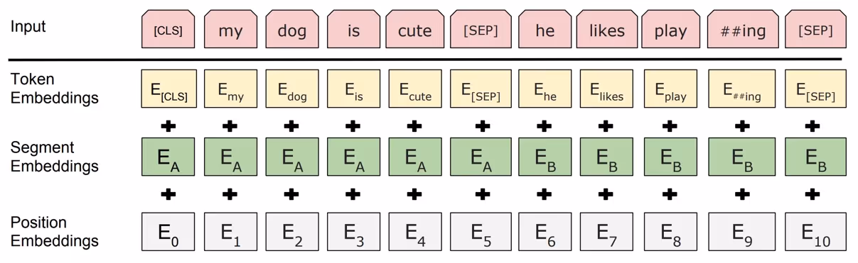
Token embedding is used to encode word tokens. Segment embedding encodes belonging to the first or to the second sentence. We preprocess input sequence the next way: if the token belongs to the first sentence, set 0, otherwise set 1. For example,
Input tokens:   [0, 6, 24, 565, 67, 0, 443, 123, 5, 6, 5, 12, 1, 1, 1]
Input Segments: [0, 0, 0, 0, 0, 0, 1, 1, 1, 1, 1, 1, 1, 1, 1]
Positional embedding encodes the position of the word in the sentence. There is an option to use embedding layer to encode positional information of token in a sequence. In the module’s code it’s done in numeric_position method. What it does is just arrange integer position.
Input tokens:   [0, 6, 24, 565, 67, 0, 443, 123, 5, 6, 5, 12, 1, 1, 1]
Input position: [0, 1, 2, 3, 4, 5, 6, 7, 8, 9, 10, 11, 12, 13, 14]
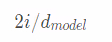
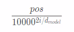
However, instead of learnable positional embedding, we use periodic functions to encode positions (as stated at [vaswani et al, 2017]).
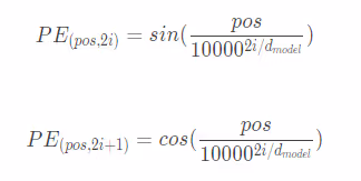
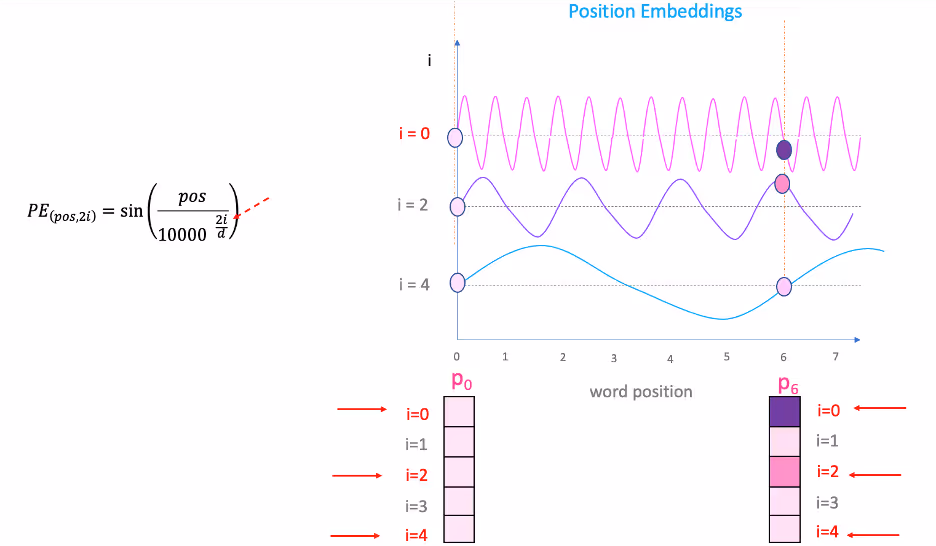
So, pos variable is the concrete value on the sin curve. i is the concrete sin curve from which to select pos. So, for i = 0 we have one periodic curve to get pos from. For i = 4 we have another.
We keep all embeddings in one module JoinEmbedding. Here is the full code for the module.
class JointEmbedding(nn.Module):

    def __init__(self, vocab_size, size):
        super(JointEmbedding, self).__init__()

        self.size = size

        self.token_emb = nn.Embedding(vocab_size, size)
        self.segment_emb = nn.Embedding(vocab_size, size)

        self.norm = nn.LayerNorm(size)

    def forward(self, input_tensor):
        sentence_size = input_tensor.size(-1)
        pos_tensor = self.attention_position(self.size, input_tensor)

        segment_tensor = torch.zeros_like(input_tensor).to(device)
        segment_tensor[:, sentence_size // 2 + 1:] = 1

        output = self.token_emb(input_tensor) + self.segment_emb(segment_tensor) + pos_tensor
        return self.norm(output)

    def attention_position(self, dim, input_tensor):
        batch_size = input_tensor.size(0)
        sentence_size = input_tensor.size(-1)

        pos = torch.arange(sentence_size, dtype=torch.long).to(device)
        d = torch.arange(dim, dtype=torch.long).to(device)
        d = (2 * d / dim)

        pos = pos.unsqueeze(1)
        pos = pos / (1e4 ** d)

        pos[:, ::2] = torch.sin(pos[:, ::2])
        pos[:, 1::2] = torch.cos(pos[:, 1::2])

        return pos.expand(batch_size, *pos.size())

    def numeric_position(self, dim, input_tensor):
        pos_tensor = torch.arange(dim, dtype=torch.long).to(device)
        return pos_tensor.expand_as(input_tensor)
As you see, from the code, we create two embedding layers
self.token_emb = nn.Embedding(vocab_size, size)
self.segment_emb = nn.Embedding(vocab_size, size)
Then in the forward method we calculate positional encoding tensor and prepare a tensor for segment Embedding
pos_tensor = self.attention_position(self.size, input_tensor)

segment_tensor = torch.zeros_like(input_tensor).to(device)
segment_tensor[:, sentence_size // 2 + 1:] = 1
Then we just sum them and pass the resulting tensor through LayerNorm.
output = self.token_emb(input_tensor) + self.segment_emb(segment_tensor) + pos_tensor
return self.norm(output)
If you want to use learnable positional embedding, you should create one more nn.Embedding instance in the constructor.
self.positional_emb = nn.Embedding(vocab_size, size)
Then in the forward method use numeric_position method to generate the input for self.positional_emb attribute.
pos_tensor = self.numeric_position(self.size, input_tensor)
...
output = self.token_emb(input_tensor) + self.segment_emb(segment_tensor) + self.positional_emb(pos_tensor)
Implementation of positional encoding in this code can be somewhat hard for understanding, so let’s review it in more details with an example.
We have a batch size of 2 and max sentence length of 5. dim attribute is the embedding size, we set it to 4. input_tensor is the word tokens tensor with size (batch_size x sentence_size), in our example, (2 x 5).
def attention_position(self, dim = 4, input_tensor):  # input_tensor shape (2 x 5)
    batch_size = 2
    sentence_size = 5
Now, we should create a vector of numerical encoding of word in a sentence.
pos = tensor([0, 1, 2, 3, 4, 5])
Vector d represents positional encoding by the embedding axis, in the formula it is
d = tensor([0, 1, 2, 3])
d = (2 * d / dim) = tensor([0, 0.5, 1, 1.5])
On the next two lines, we see the process that is called Broadcasting. PyTorch’s broadcasting is strongly inspired by NumPy (read more on NumPy Broadcasting).
Firstly, we unsqueeze pos vector to the shape (5 x 1). Then we multiply it position-wise with d vector using PyTorch broadcasting. Relating to the formula we’re calculating a value that we pass further to periodic function
pos = pos.unsqueeze(1) = tensor([[0],
                                 [1],
                                 [2],
                                 [3],
                                 [4]])

pos = pos / (1e4 ** d) = size (5 x 4) =
= tensor([[0.0000e+00, 0.0000e+00, 0.0000e+00, 0.0000e+00],
          [1.0000e+00, 1.0000e-02, 1.0000e-04, 1.0000e-06],
          [2.0000e+00, 2.0000e-02, 2.0000e-04, 2.0000e-06],
          [3.0000e+00, 3.0000e-02, 3.0000e-04, 3.0000e-06],
          [4.0000e+00, 4.0000e-02, 4.0000e-04, 4.0000e-06]])
A final operation is just to apply periodic functions to this pos tensor.
pos[:, ::2] = torch.sin(pos[:, ::2])    # Apply to 2i
pos[:, 1::2] = torch.cos(pos[:, 1::2])  # Apply to 2i + 1
And extending pos on every element in batch.
return pos.expand(batch_size, *pos.size()) = size (2 x 5 x 4)
The returned tensor has the same size as our other embeddings. We just simulated embedding layer with simple mathematical operations.
AttentionHead
Attention is the heart of transformers. This is exactly what makes transformers so good. BERT uses the mechanism called self-attention. It is well described in this article Illustrated: Self-Attention. And a quote from this resource
A self-attention module takes in n inputs and returns n outputs. What happens in this module? In layman’s terms, the self-attention mechanism allows the inputs to interact with each other (“self”) and find out who they should pay more attention to (“attention”). The outputs are aggregates of these interactions and attention scores.
There are various types of attentions that can be used. We use the one from [vaswani et al, 2017].
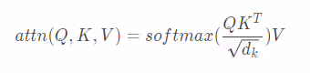
where Q is query, K is key, and V is value.
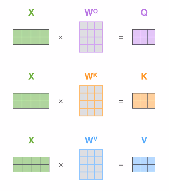
For each of them we create linear layer with trainable weights. So, we’ll teach the network to ‘pay attention’. On the pictures below, you may see the visualization of attention multiplication. That’s exactly what we do in the code.
class AttentionHead(nn.Module):

    def __init__(self, dim_inp, dim_out):
        super(AttentionHead, self).__init__()

        self.dim_inp = dim_inp

        self.q = nn.Linear(dim_inp, dim_out)
        self.k = nn.Linear(dim_inp, dim_out)
        self.v = nn.Linear(dim_inp, dim_out)

    def forward(self, input_tensor: torch.Tensor, attention_mask: torch.Tensor = None):
        query, key, value = self.q(input_tensor), self.k(input_tensor), self.v(input_tensor)

        scale = query.size(1) ** 0.5
        scores = torch.bmm(query, key.transpose(1, 2)) / scale

        scores = scores.masked_fill_(attention_mask, -1e9)
        attn = f.softmax(scores, dim=-1)
        context = torch.bmm(attn, value)

        return context
As you see in the __init__, we create linear module for query, key, and value. For simplicity in this tutorial they all have same shapes.
Let’s continue above’s example. dim_inp is the size of embedding and equals to 4. Let’s take hidden attention size dim_out as 6.
Let’s follow the forward method step by step. Instead of printing the values of tensors we’ll just print their sizes (shapes).
# input tensor is the output of JointEmbedding module
# attention mask is the vector that masks [PAD] tokens
def forward(self, input_tensor: size (2 x 5 x 4), attention_mask: size (2 x 1 x 5)):
First thing we do is calculate query, key, value tensors
query, key, value = size (2 x 5 x 6), size (2 x 5 x 6), size (2 x 5 x 6)
Further, we calculate scaled multiplication of query and key.
scale = query.size(1) ** 0.5
scores = torch.bmm(query, key.transpose(1, 2)) / scale = size (2 x 5 x 5)
torch.bmm is batched matrix multiplication function. This multiplies each matrix in a batch, skipping the first axis. transpose method transposes tensor for 2 specific dimensions.
We don’t want our model to ‘pay attention’ on [PAD] tokens at all. This is why we have attention mask vector. Using this vector we shadow the scores of [PAD] tokens.
scores = scores.masked_fill_(attention_mask, -1e9) = size (2 x 5 x 5)
Now, we calculate the attention context itself.
attn = f.softmax(scores, dim=-1) = size (2 x 5 x 5)
context = torch.bmm(attn, value) = size (2 x 5 x 6)
So, each input value was weighted by the attention tensor.
MultiHeadAttention
Single attention layer (head) is restricted to learn only the information from one particular subspace. Multi-head attention is the set of parallel attention heads that learns to retrieve the information from different representations. You may look on them as on filters in Convolutional Neural Networks.
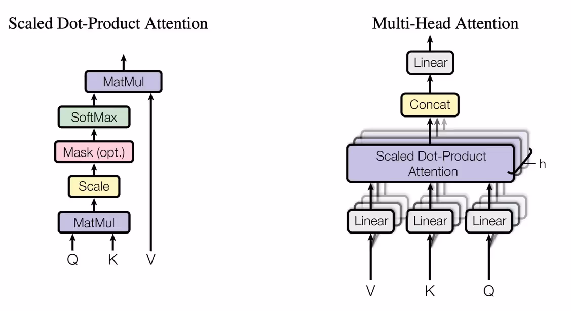
You may see how it works on the visualization of two-head attention on a picture below. We print the attentions for the word it. The first attention (orange) scores word animal the most while the second attention (green) scores word tired the most.
Let’s back to our code. As always, here is the full code of the module, then we go through it step by step
class MultiHeadAttention(nn.Module):

    def __init__(self, num_heads, dim_inp, dim_out):
        super(MultiHeadAttention, self).__init__()

        self.heads = nn.ModuleList([
            AttentionHead(dim_inp, dim_out) for _ in range(num_heads)
        ])
        self.linear = nn.Linear(dim_out * num_heads, dim_inp)
        self.norm = nn.LayerNorm(dim_inp)

    def forward(self, input_tensor: torch.Tensor, attention_mask: torch.Tensor):
        s = [head(input_tensor, attention_mask) for head in self.heads]
        scores = torch.cat(s, dim=-1)
        scores = self.linear(scores)
        return self.norm(scores)
dim_inp and dim_out had the same values as in AttentionHead paragraph: dim_inp equals to 4, dim_out equals to 6. num_heads is 3. For simplicity, we use output size of linear layer the same as embedding size.
self.linear = nn.Linear(dim_out * num_heads, dim_inp) = nn.Linear(4 * 3, 4)
So, input size of linear layer is 12, output is 4.
The forward method has the same arguments as the AttentionHead.
def forward(self, input_tensor: size (2 x 5 x 4), attention_mask: size (2 x 1 x 5)):
At the first operation we calculate the list of attentions s.
s = [head(input_tensor, attention_mask) for head in self.heads]
s = [
    tensor(2 x 5 x 6),
    tensor(2 x 5 x 6),
    tensor(2 x 5 x 6),
]
Further, we concatenate tensors by the last axis.
scores = torch.cat(s, dim=-1) = tensor(2 x 5 x 18)
Pass scores through linear layer and normalize.
scores = self.linear(scores) = tensor(2 x 5 x 4)
return self.norm(scores)
Encoder
Encoder consists of multi-head attention and feed-forward neural network. In original Attention Is All You Need, the stack of identical encoder layers is used. We use only one in this tutorial because of lazyness for simplicity.
Encoder layer diagram from [vaswani et al, 2017].
class Encoder(nn.Module):

    def __init__(self, dim_inp, dim_out, attention_heads=4, dropout=0.1):
        super(Encoder, self).__init__()

        self.attention = MultiHeadAttention(attention_heads, dim_inp, dim_out)
        self.feed_forward = nn.Sequential(
            nn.Linear(dim_inp, dim_out),
            nn.Dropout(dropout),
            nn.GELU(),
            nn.Linear(dim_out, dim_inp),
            nn.Dropout(dropout)
        )
        self.norm = nn.LayerNorm(dim_inp)

    def forward(self, input_tensor: torch.Tensor, attention_mask: torch.Tensor):
        context = self.attention(input_tensor, attention_mask)
        res = self.feed_forward(context)
        return self.norm(res)
Feed forward network should be explained such as it’s slightly different than the one you may see in Attention Is All You Need.
self.feed_forward = nn.Sequential(
    nn.Linear(dim_inp, dim_out),
    nn.Dropout(dropout),
    nn.GELU(),
    nn.Linear(dim_out, dim_inp),
    nn.Dropout(dropout)
)
Original encoder has RelU as activation function. We use GelU (read more Gaussian Error Linear Units (Gelus)).

Visualization of GelU function comparing to RelU and ELU from [hendrycks et al, 2016].
The formula representation of our feed forward network.
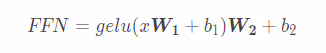
Also, we add dropout layer after each linear.
Why we use GelU? Just because it give better results. You may follow Searching for Activation Functions paper for more details.
The forward method does simple:
- Calculate attention context
- Pass context through feed forward network
- Normalize
def forward(self, input_tensor: torch.Tensor, attention_mask: torch.Tensor):
    context = self.attention(input_tensor, attention_mask)
    res = self.feed_forward(context)
    return self.norm(res)
BERT
BERT module is a container that combines all the modules together and returns the output.
class BERT(nn.Module):

    def __init__(self, vocab_size, dim_inp, dim_out, attention_heads=4):
        super(BERT, self).__init__()

        self.embedding = JointEmbedding(vocab_size, dim_inp)
        self.encoder = Encoder(dim_inp, dim_out, attention_heads)

        self.token_prediction_layer = nn.Linear(dim_inp, vocab_size)
        self.softmax = nn.LogSoftmax(dim=-1)
        self.classification_layer = nn.Linear(dim_inp, 2)

    def forward(self, input_tensor: torch.Tensor, attention_mask: torch.Tensor):
        embedded = self.embedding(input_tensor)
        encoded = self.encoder(embedded, attention_mask)

        token_predictions = self.token_prediction_layer(encoded)

        first_word = encoded[:, 0, :]
        return self.softmax(token_predictions), self.classification_layer(first_word)
We use linear layer (and softmax) with output that is equal to the vocabulary size for token prediction task.
self.token_prediction_layer = nn.Linear(dim_inp, vocab_size)
self.softmax = nn.LogSoftmax(dim=-1)
And linear layer with output of 2 for next sentence prediction task
self.classification_layer = nn.Linear(dim_inp, 2)
The output of the network
argmax(NSP output) = [1, 0] is NOT next sentence
argmax(NSP output) = [0, 1] is next sentence
Everything is simple in the forward. At first we calculate embedding, then pass embeddings to our encoder.
embedded = self.embedding(input_tensor)
encoded = self.encoder(embedded, attention_mask)
Secondly, we calculate the model output.
token_predictions = self.token_prediction_layer(encoded)

first_word = encoded[:, 0, :]
return self.softmax(token_predictions), self.classification_layer(first_word)
The full model graph is also available. To build the graph, run the script graph.py. It saves the graph to data/logs directory. Run tensorboard
tensorboard --logdir data/logs
Open http://localhost:6006 in the browser, go to Graph tab. You should see the graph of our BERT model.

Train the model
All training operations are in bert.trainer module in BertTrainer class. Let’s take a look at the class constructor.
class BertTrainer:

    def __init__(self,
                 model: BERT,
                 dataset: IMDBBertDataset,
                 log_dir: Path,
                 checkpoint_dir: Path = None,
                 print_progress_every: int = 10,
                 print_accuracy_every: int = 50,
                 batch_size: int = 24,
                 learning_rate: float = 0.005,
                 epochs: int = 5,
                 ):
        self.model = model
        self.dataset = dataset

        self.batch_size = batch_size
        self.epochs = epochs
        self.current_epoch = 0

        self.loader = DataLoader(self.dataset, batch_size=self.batch_size, shuffle=True)

        self.writer = SummaryWriter(str(log_dir))
        self.checkpoint_dir = checkpoint_dir

        self.criterion = nn.BCEWithLogitsLoss().to(device)
        self.ml_criterion = nn.NLLLoss(ignore_index=0).to(device)
        self.optimizer = torch.optim.Adam(model.parameters(), lr=learning_rate, weight_decay=0.015)
Then we shadow other than [MASK] tokens in model output token. Reason for that is that we train model to predict only [MASK] tokens.
tm = inverse_token_mask.unsqueeze(-1).expand_as(token)
token = token.masked_fill(tm, 0)
Further we calculate criterions and sum the loss.
loss_token = self.ml_criterion(token.transpose(1, 2), token_target)
loss_nsp = self.criterion(nsp, nsp_target)

loss = loss_token + loss_nsp
average_nsp_loss += loss_nsp
average_mlm_loss += loss_token
Make backward step and update weights.
loss.backward()
self.optimizer.step()
From time to time, we calculate model’s accuracy
if index % self._accuracy_every == 0:
    s += self.accuracy_summary(index, token, nsp, token_target, nsp_target)
It calculates MLM and NSP accuracies
nsp_acc = nsp_accuracy(nsp, nsp_target)
token_acc = token_accuracy(token, token_target, inverse_token_mask)
For NSP we calculate how much tensors in a batch were predicted correctly.
def nsp_accuracy(result: torch.Tensor, target: torch.Tensor):
    s = (result.argmax(1) == target.argmax(1)).sum()
    return round(float(s / result.size(0)), 2)
For MLM we should do some manipulations — apply masking to the model output and target. Or as we do in the code, just select masked tokens and compare.
def token_accuracy(result: torch.Tensor, target: torch.Tensor, inverse_token_mask: torch.Tensor):
    r = result.argmax(-1).masked_select(~inverse_token_mask)
    t = target.masked_select(~inverse_token_mask)
    s = (r == t).sum()
    return round(float(s / (result.size(0) * result.size(1))), 2)
Training Results and Summary
Finally, we are ready to run the training of our model. Long story short, open the main.py script file, check the learning parameters and run.
I trained the model on nVidia GeForce 1050ti GPU. If cuda is supported, the model will be trained on GPU by default. The next parameters of model were used
EMB_SIZE = 64
HIDDEN_SIZE = 36
EPOCHS = 4
BATCH_SIZE = 12
NUM_HEADS = 4
Embedding size is 64, hidden attention context size is 36, batch size is 12, number of attention heads is 4, and number of encoders is 1. Learning rate is 7e-5.
We use TensorBoard to track the training process.
After you run the training script, you should see how it prepares the IMDB dataset
Prepare dataset
Create vocabulary
100%|██████████| 491161/491161 [00:05<00:00, 93957.36it/s]
Preprocessing dataset
100%|██████████| 50000/50000 [00:35<00:00, 1407.99it/s]
Then the trainer prints the model summary
Model Summary

===================================
Device: cuda
Training dataset len: 882322
Max / Optimal sentence len: 27
Vocab size: 71942
Batch size: 12
Batched dataset len: 73526
===================================
And the training begins
Begin epoch 0
00:00:02 | Epoch 1 | 20 / 73526 (0.03%) | NSP loss   0.72 | MLM loss  11.25
00:00:04 | Epoch 1 | 40 / 73526 (0.05%) | NSP loss   0.70 | MLM loss  11.22
00:00:06 | Epoch 1 | 60 / 73526 (0.08%) | NSP loss   0.70 | MLM loss  11.13
00:00:08 | Epoch 1 | 80 / 73526 (0.11%) | NSP loss   0.71 | MLM loss  11.13
00:00:11 | Epoch 1 | 100 / 73526 (0.14%) | NSP loss   0.69 | MLM loss  11.05
00:00:13 | Epoch 1 | 120 / 73526 (0.16%) | NSP loss   0.70 | MLM loss  10.98
00:00:15 | Epoch 1 | 140 / 73526 (0.19%) | NSP loss   0.69 | MLM loss  10.95
00:00:18 | Epoch 1 | 160 / 73526 (0.22%) | NSP loss   0.70 | MLM loss  10.90
00:00:20 | Epoch 1 | 180 / 73526 (0.24%) | NSP loss   0.71 | MLM loss  10.89
00:00:22 | Epoch 1 | 200 / 73526 (0.27%) | NSP loss   0.72 | MLM loss  10.83 | NSP accuracy 0.25 | Token accuracy 0.01
The BERT model and even our too much simplified BERT model converges slowly and requires a lot of computational resources. I was able to train only one epoch. That took a little bit more than two hours
02:20:49 | Epoch 1 | 73440 / 73526 (99.88%) | NSP loss   0.69 | MLM loss   4.49
02:20:52 | Epoch 1 | 73460 / 73526 (99.91%) | NSP loss   0.69 | MLM loss   4.37
02:20:54 | Epoch 1 | 73480 / 73526 (99.94%) | NSP loss   0.69 | MLM loss   4.24
02:20:56 | Epoch 1 | 73500 / 73526 (99.96%) | NSP loss   0.69 | MLM loss   4.38
02:20:59 | Epoch 1 | 73520 / 73526 (99.99%) | NSP loss   0.70 | MLM loss   4.37
Let’s take a look how the loss value was changed throughout a time

Change of MLM loss with time.
You may see that our BERT model’s loss really converges to some minimum but this process is really slow. For example here is the log message on 44’s % of data processed
01:03:01 | Epoch 1 | 32880 / 73526 (44.72%) | NSP loss 0.69 | MLM loss 4.78
And the message on 100’s % of data processed
02:20:59 | Epoch 1 | 73520 / 73526 (99.99%) | NSP loss 0.70 | MLM loss 4.37
For an hour of training the NSP loss was reduced only on some tenth parts.

Change of NSP loss with time.
From the chart above you could say that NSP loss doesn’t converge but diverges. It converges but even slower than MLM. We can see this if we apply smoothing to the values of this chart

Smoothed change of NSP loss with time.
I would say we have such result because of our dataset. We use IMDB reviews for training and splitted text on sentences by . symbol. Now, I ask you to take a look what these sentences are. Noticed? So, it’s hard for the model to have a good catch on the data to solve this task. Original BERT used English Wikipedia and Books Corpus with good, long, and informative sentences.
Let’s take a look how train accuracies changes throughout a time.

Change of MLM training accuracy.

Change of NSP training accuracy.
The accuracy actually correlate with the loss. When MLM loss is slightly reduced, MLM accuracy is slightly improved. NSP accuracy is even more wiggy and after the first epoch is slightly more than 0.5 in average. The conclusion is that we definitely need to try different dataset. But anyway that is still good results for a tutorial :)
The model built in this tutorial is not the full BERT. In best words it’s just simplified version of BERT that is good only to understand its architecture, how it works. There are a lot of pre-trained BERT (and its variants) models build by HuggingFace. Now, you should have the understanding of how to build BERT from scratch (with pyTorch of course). Further, you can try to use different datasets and model parameters in order to see if it gives better results of tasks, especially, NSP task convergence.


.avif)


.avif)
.avif)


We are interested in your opinion